News

How its work : Timer

What is the difference between On Delay, Off Delay, Single Shot, Interval On and all these other time delay functions?

Solution/Resolution:

Understanding the differences between all the functions available in time delay relays can sometimes be a daunting task. When designing circuits using time delay relays, questions such as what initiates a time delay relay, does the timing start with the application or release of voltage, when is the output relay energized, etc., must be asked.

Time delay relays are simply control relays with a time delay built in. Their purpose is to control an event based on time. The difference between relays and time delay relays is when the output contacts open & close: on a control relay, it happens when voltage is applied and removed from the coil; on time delay relays, the contacts can open or close before or after some time delay.

Typically, time delay relays are initiated or triggered by one of two methods:

• application of input voltage
• opening or closing of a trigger signal

These trigger signals can be one of two designs:

• a control switch (dry contact), i.e., limit switch, push button, float switch, etc.
• voltage (commonly known as a power trigger)

CAUTION: any time delay relay that is designed to be initiated with a dry contact control switch trigger could be damaged if voltage is applied to the trigger switch terminals.  Only products that have a "power trigger" should be used with voltage as the trigger.

To help understand, some definitions are important:

• Input Voltage-control voltage applied to the input terminals. Depending on the function, input voltage will either initiate the unit or make it ready to initiate when a trigger is applied.
• Trigger Signal-on certain timing functions, a trigger is used to initiate the unit after input voltage has been applied. As noted above, this trigger can either be a control switch (dry contact switch) or a power trigger (voltage).
• Output (Load)-every time delay relay has an output (either mechanical relay or solid state) that will open & close to control the load. Note that the user must provide the voltage to power the load being switched by the output contacts of the time delay relay.

Below are both written and visual descriptions on how the common timing functions operate. A Timing Chart shows the relationship between Input Voltage, Trigger (if present) and Output. 

Function	Operation	Timing Chart
ON DELAY Delay on Make Delay on Operate	Upon application of input voltage, the time delay (t) begins. At the end of the time delay (t), the output is energized. Input voltage must be removed to reset the time delay relay & de-energize the output.
INTERVAL ON Interval	Upon application of input voltage, the output is energized and the time delay (t) begins. At the end of the time delay (t), the output is de-energized. Input voltage must be removed to reset the time delay relay.
OFF DELAY Delay on Release Delay on Break Delay on De-Energization	Upon application of input voltage, the time delay relay is ready to accept a trigger. When the trigger is applied, the output is energized. Upon removal of the trigger, the time delay (t) begins. At the end of the time delay (t), the output is de-energized. Any application of the trigger during the time delay will reset the time delay (t) and the output remains energized.
SINGLE SHOT One Shot Momentary Interval	Upon application of input voltage, the time delay relay is ready to accept a trigger. When the trigger is applied, the output is energized and the time delay (t) begins. During the time delay (t), the trigger is ignored. At the end of the time delay (t), the output is de-energized and the time delay relay is ready to accept another trigger.
FLASHER (Off First)	Upon application of input voltage, the time delay (t) begins. At the end of the time delay (t), the output is energized and remains in that condition for the time delay (t). At the end of the time delay (t), the output is de-energized and the sequence repeats until input voltage is removed.
FLASHER (On First)	Upon application of input voltage, the output is energized and the time delay (t) begins. At the end of the time delay (t), the output is de-energized and remains in that condition for the time delay (t). At the end of the time delay (t), the output is energized and the sequence repeats until input voltage is removed.
ON/OFF DELAY	Upon application of input voltage, the time delay relay is ready to accept a trigger. When the trigger is applied, the time delay (t1) begins. At the end of the time delay (t1), the output is energized. When the trigger is removed, the output contacts remain energized for the time delay (t2). At the end of the time delay (t2), the output is de-energized & the time delay relay is ready to accept another trigger. If the trigger is removed during time delay period (t1), the output will remain de-energized and time delay (t1) will reset. If the trigger is re-applied during time delay period (t2), the output will remain energized and the time delay (t2) will reset.
SINGLE SHOT FALLING EDGE	Upon application of input voltage, the time delay relay is ready to accept a trigger. When the trigger is applied, the output remains de-energized. Upon removal of the trigger, the output is energized and the time delay (t) begins. At the end of the time delay (t), the output is de-energized unless the trigger is removed and re-applied prior to time out (before time delay (t) elapses). Continuous cycling of the trigger at a rate faster than the time delay (t) will cause the output to remain energized indefinitely.
WATCHDOG Retriggerable Single Shot	Upon application of input voltage, the time delay relay is ready to accept a trigger. When the trigger is applied, the output is energized and the time delay (t) begins. At the end of the time delay (t), the output is de-energized unless the trigger is removed and re-applied prior to time out (before time delay (t) elapses). Continuous cycling of the trigger at a rate faster than the time delay (t) will cause the output to remain energized indefinitely.
TRIGGERED ON DELAY	Upon application of input voltage, the time delay relay is ready to accept a trigger. When the trigger is applied, the time delay (t) begins. At the end of the time delay (t), the output is energized and remains in that condition as long as either the trigger is applied or the input voltage remains. If the trigger is removed during the time delay (t), the output remains de-energized & the time delay (t) is reset.
REPEAT CYCLE (OFF 1st)	Upon application of input voltage, the time delay (t1) begins. At the end of the time delay (t1), the output is energized and remains in that condition for the time delay (t2). At the end of this time delay, the output is de-energized and the sequence repeats until input voltage is removed.
REPEAT CYCLE (ON 1st)	Upon application of input voltage, the output is energized and the time delay (t1) begins. At the end of the time delay (t1), the output is de-energized and remains in that condition for the time delay (t2). At the end of this time delay, the output is energized and the sequence repeats until input voltage is removed.
DELAYED INTERVAL Single Cycle	Upon application of input voltage, the time delay (t1) begins. At the end of the time delay (t1), the output is energized and remains in that condition for the time delay (t2). At the end of this time delay (t2), the output is de-energized. Input voltage must be removed to reset the time delay relay.
TRIGGERED DELAYED INTERVAL Single Cycle	Upon application of input voltage, the time delay relay is ready to accept a trigger. When the trigger is applied, the time delay (t1) begins. At the end of the time delay (t1), the output is energized and remains in that condition for the time delay (t2). At the end of the time delay (t2), the output is de-energized & the relay is ready to accept another trigger. During both time delay (t1) & time delay (t2), the trigger is ignored.
TRUE OFF DELAY	Upon application of input voltage, the output is energized. When the input voltage is removed, the time delay (t) begins. At the end of the time delay (t), the output is de-energized. Input voltage must be applied for a minimum of 0.5 seconds to assure proper operation. Any application of the input voltage during the time delay (t) will reset the time delay. No external trigger is required.
ON DELAY/ TRUE OFF DELAY	Upon application of input voltage, the time delay (t1) begins. At the end of the time delay (t1), the output is energized. When the input voltage is removed, the output remains energized for the time delay (t2). At the end of the time delay (t2), the output is de-energized. Input voltage must be applied for a minimum of 0.5 seconds to assure proper operation. Any application of the input voltage during the time delay (t2) will keep the output energized & reset the time delay (t2). No external trigger is required.
SINGLE SHOT-FLASHER	Upon application of input voltage, the time delay relay is ready to accept a trigger. When the trigger is applied, the time delay (t1) begins and the output is energized for the time delay (t2). At the end of this time delay (t2), the output is de-energized and remains in that condition for the time delay (t2). At the end of the time delay (t2), the output is energized and the sequence repeats until time delay (t1) is completed. During the time delay (t1), the trigger is ignored.
ON DELAY-FLASHER	Upon application of input voltage, the time delay begins (t1). At the end of the time delay (t1), the output is energized and remains in that condition for the time delay (t2). At the end of this time delay (t2), the output is de-energized and remains in that condition for the time delay (t2). At the end of the time delay (t2), the output is energized and the sequence repeats until input voltage is removed.
PERCENTAGE	Upon initial application of input voltage, the output is energized and time delay (t1) begins. Time Delay (t1) is adjustable as a percentage of the overall cycle time (t2). At the end of time delay (t1), the output is de-energized for the remainder of overall cycle (t2-t1). The sequence then repeats until input voltage is removed. If input voltage is removed and reapplied, the timing cycle will continue from where it left off when the input voltage was removed. A setting of 100% energizes the output continuously while a setting of 0% de-energizes the output continuously.
PERCENTAGE (NO MEMORY)	Upon initial application of input voltage, the output is energized and time delay (t1) begins. Time Delay (t1) is adjustable as a percentage if the overall cycle time (t2). At the end of time delay (t1), the output is de-energized for the remainder of overall cycle (t2-t1). The sequence then repeats until input voltage is removed. If input voltage is removed and reapplied, the timing cycle will be reset. A setting of 100% energizes the output continuously while a setting of 0% de-energizes the output continuously.

3JIndustry Specialized Distributor - Buy & Sales Used Products

Email : Sales@3JIndustry.com

How its Work : Inductive - Capacitive - Photoelectric - Ultrasonic sensors

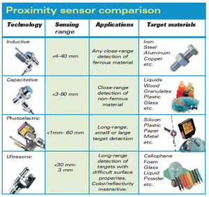
11Proximity sensors detect the presence or absence of objects using electromagnetic fields, light, and sound. There are many types, each suited to specific applications and environments.

Inductive sensors

These non-contact proximity sensors detect ferrous targets, ideally mild steel thicker than one millimeter. They consist of four major components: a ferrite core with coils, an oscillator, a Schmitt trigger, and an output amplifier. The oscillator creates a symmetrical, oscillating magnetic field that radiates from the ferrite core and coil array at the sensing face. When a ferrous target enters this magnetic field, small independent electrical currents called eddy currents are induced on the metal’s surface. This changes the reluctance (natural frequency) of the magnetic circuit, which in turn reduces the oscillation amplitude. As more metal enters the sensing field the oscillation amplitude shrinks, and eventually collapses. (This is the “Eddy Current Killed Oscillator” or ECKO principle.) The Schmitt trigger responds to these amplitude changes, and adjusts sensor output. When the target finally moves from the sensor’s range, the circuit begins to oscillate again, and the Schmitt trigger returns the sensor to its previous output.

If the sensor has a normally open configuration, its output is anon signal when the target enters the sensing zone. With normally closed, its output is an off signal with the target present. Output is then read by an external control unit (e.g. PLC, motion controller, smart drive) that converts the sensor on and off states into useable information. Inductive sensors are typically rated by frequency, or on/off cycles per second. Their speeds range from 10 to 20 Hz in ac, or 500 Hz to 5 kHz in dc. Because of magnetic field limitations, inductive sensors have a relatively narrow sensing range — from fractions of millimeters to 60 mm on average — though longer-range specialty products are available.

To accommodate close ranges in the tight confines of industrial machinery, geometric and mounting styles available include shielded (flush), unshielded (non-flush), tubular, and rectangular “flat-pack”. Tubular sensors, by far the most popular, are available with diameters from 3 to 40 mm.

But what inductive sensors lack in range, they make up in environment adaptability and metal-sensing versatility. With no moving parts to wear, proper setup guarantees long life. Special designs with IP ratings of 67 and higher are capable of withstanding the buildup of contaminants such as cutting fluids, grease, and non-metallic dust, both in the air and on the sensor itself. It should be noted that metallic contaminants (e.g. filings from cutting applications) sometimes affect the sensor’s performance. Inductive sensor housing is typically nickel-plated brass, stainless steel, or PBT plastic.

Capacitive sensors

Capacitive proximity sensors can detect both metallic and non-metallic targets in powder, granulate, liquid, and solid form. This, along with their ability to sense through nonferrous materials, makes them ideal for sight glass monitoring, tank liquid level detection, and hopper powder level recognition.

In capacitive sensors, the two conduction plates (at different potentials) are housed in the sensing head and positioned to operate like an open capacitor. Air acts as an insulator; at rest there is little capacitance between the two plates. Like inductive sensors, these plates are linked to an oscillator, a Schmitt trigger, and an output amplifier. As a target enters the sensing zone the capacitance of the two plates increases, causing oscillator amplitude change, in turn changing the Schmitt trigger state, and creating an output signal. Note the difference between the inductive and capacitive sensors: inductive sensors oscillate until the target is present and capacitive sensors oscillate when the target is present.

Because capacitive sensing involves charging plates, it is somewhat slower than inductive sensing ... ranging from 10 to 50 Hz, with a sensing scope from 3 to 60 mm. Many housing styles are available; common diameters range from 12 to 60 mm in shielded and unshielded mounting versions. Housing (usually metal or PBT plastic) is rugged to allow mounting very close to the monitored process. If the sensor has normally-open and normally-closed options, it is said to have a complimentary output. Due to their ability to detect most types of materials, capacitive sensors must be kept away from non-target materials to avoid false triggering. For this reason, if the intended target contains a ferrous material, an inductive sensor is a more reliable option.

Photoelectric sensors

Photoelectric sensors are so versatile that they solve the bulk of problems put to industrial sensing. Because photoelectric technology has so rapidly advanced, they now commonly detect targets less than 1 mm in diameter, or from 60 m away. Classified by the method in which light is emitted and delivered to the receiver, many photoelectric configurations are available. However, all photoelectric sensors consist of a few of basic components: each has an emitter light source (Light Emitting Diode, laser diode), a photodiode or phototransistor receiver to detect emitted light, and supporting electronics designed to amplify the receiver signal. The emitter, sometimes called the sender, transmits a beam of either visible or infrared light to the detecting receiver.

All photoelectric sensors operate under similar principles. Identifying their output is thus made easy; darkon and light-on classifications refer to light reception and sensor output activity. If output is produced when no light is received, the sensor is dark-on. Output from light received, and it’s light-on. Either way, deciding on light-on or dark-on prior to purchasing is required unless the sensor is user adjustable. (In that case, output style can be specified during installation by flipping a switch or wiring the sensor accordingly.)

Through-beam

The most reliable photoelectric sensing is with through-beam sensors. Separated from the receiver by a separate housing, the emitter provides a constant beam of light; detection occurs when an object passing between the two breaks the beam. Despite its reliability, through-beam is the least popular photoelectric setup. The purchase, installation, and alignment

of the emitter and receiver in two opposing locations, which may be quite a distance apart, are costly and laborious. With newly developed designs, through-beam photoelectric se

nsors typically offer the longest sensing distance of photoelectric sensors — 25 m and over is now commonplace. New laser diode emitter models can transmit a well-collimated beam 60 m for increased accuracy and detection. At these distances, some through-beam laser sensors are capable of detecting an object the size of a fly; at close range, that becomes 0.01 mm. But while these laser sensors increase precision, response speed is the same as with non-laser sensors — typically around 500 Hz.

One ability unique to throughbeam photoelectric sensors is effective sensing in the presence of thick airborne contaminants. If pollutants build up directly on the emitter or receiver, there is a higher probability of false triggering. However, some manufacturers now incorporate alarm outputs into the sensor’s circuitry that monitor the amount of light hitting the receiver. If detected light decreases to a specified level without a target in place, the sensor sends a warning by means of a builtin LED or output wire.

Through-beam photoelectric sensors have commercial and industrial applications. At home, for example, they detect obstructions in the path of garage doors; the sensors have saved many a bicycle and car from being smashed. Objects on industrial conveyors, on the other hand, can be detected anywhere between the emitter and receiver, as long as there are gaps between the monitored objects, and sensor light does not “burn through” them. (Burnthrough might happen with thin or lightly colored objects that allow emitted light to pass through to the receiver.)

Retro-reflective

Retro-reflective sensors have the next longest photoelectric sensing distance, with some units capable of monitoring ranges up to 10 m. Operating similar to through-beam sensors without reaching the same sensing distances, output occurs when a constant beam is broken. But instead of separate housings for emitter and receiver, both are located in the same housing, facing the same direction. The emitter produces a laser, infrared, or visible light beam and projects it towards a specially designed reflector, which then deflects the beam back to the receiver. Detection occurs when the light path is broken or otherwise disturbed.

One reason for using a retro-reflective sensor over a through-beam sensor is for the convenience of one wiring location; the opposing side only requires reflector mounting. This results in big cost savings in both parts and time. However, very shiny or reflective objects like mirrors, cans, and plastic-wrapped juice boxes create a challenge for retro-reflective photoelectric sensors. These targets sometimes reflect enough light to trick the receiver into thinking the beam was not interrupted, causing erroneous outputs.

Some manufacturers have addressed this problem with polarization filtering, which allows detection of light only from specially designed reflectors ... and not erroneous target reflections.

Diffuse

As in retro-reflective sensors, diffuse sensor emitters and receivers are located in the same housing. But the target acts as the reflector, so that detection is of light reflected off the dist

urbance object. The emitter sends out a beam of light (most often a pulsed infrared, visible red, or laser) that diffuses in all directions, filling a detection area. The target then enters the area and deflects part of the beam back to the receiver. Detection occurs and output is turned on or off (depending upon whether the sensor is light-on or dark-on) when sufficient light falls on the receiver.

Diffuse sensors can be found on public washroom sinks, where they control automatic faucets. Hands placed under the spray head act as reflector, triggering (in this case) the opening of a water valve. Because the target is the reflector, diffuse photoelectric sensors are often at the mercy of target material and surface properties; a non-reflective target such as matte-black paper will have a significantly decreased sensing range as compared to a bright white target. But what seems a drawback ‘on the surface’ can actually be useful.

Because diffuse sensors are somewhat color dependent, certain versions are suitable for distinguishing dark and light targets in applications that require sorting or quality control by contrast. With only the sensor itself to mount, diffuse sensor installation is usually simpler than with through-beam and retro-reflective types. Sensing distance deviation and false triggers caused by reflective backgrounds led to the development of diffuse sensors that focus; they “see” targets and ignore background.

There are two ways in which this is achieved; the first and most common is through fixed-field technology. The emitter sends out a beam of light, just like a standard diffuse photoelectric sensor, but for two receivers. One is focused on the desired sensing sweet spot, and the other on the long-range background. A comparator then determines whether the long-range receiver is detecting light of higher intensity than what is being picking up the focused receiver. If so, the output stays off. Only when focused receiver light intensity is higher will an output be produced.

The second focusing method takes it a step further, employing an array of receivers with an adjustable sensing distance. The device uses a potentiometer to electrically adjust the sensing range. Such sensor

s operate best at their preset sweet spot. Allowing for small part recognition, they also provide higher tolerances in target area cutoff specifications and improved colorsensing capabilities. However, target surface qualities, such as glossiness, can produce varied results. In addition, highly reflective objects outside the sensing area tend to send enough light back to the receivers for an output, especially when the receivers are electrically adjusted.

To combat these limitations, some sensor manufacturers developed a technology known as true background suppression by triangulation.

A true background suppression sensor emits a beam of light exactly like a standard, fixed-field diffuse sensor. But instead of detecting light intensity, background suppression units rely completely on the angle at which the beam returns to the sensor.

To accomplish this, background suppression sensors use two (or more) fixed receivers accompanied by a focusing lens. The angle of received light is mechanically adjusted, allowing for a steep cutoff between target and background ... sometimes as small as 0.1 mm. This is a more stable method when reflective backgrounds are present, or when target color variations are an issue; reflectivity and color affect the intensity of reflected light, but not the angles of refraction used by triangulation- based background suppression photoelectric sensors.

Ultrasonic sensors

Ultrasonic proximity sensors are used in many automated production processes. They employ sound waves to detect objects, so color and transparency do not affect them (though extreme textures might). This makes them ideal for a variety of applications, including the longrange detection of clear glass and plastic, distance measurement, continuous fluid and granulate level control, and paper, sheet metal, and wood stacking.

The most common configurations are the same as in photoelectric sensing: through beam, retro-reflective, and diffuse versions. Ultrasonic diffuse proximity sensors employ a sonic transducer, which emits a series of sonic pulses, then listens for their return from the reflecting target. Once the reflected signal is received, the sensor signals an output to a control device. Sensing ranges extend to 2.5 m. Sensitivity, defined as the time window for listen cycles versus send or chirp cycles, may be adjusted via a teach-in button or potentiometer. While standard diffuse ultrasonic sensors give a simple present/absent output, some produce analog signals, indicating distance with a 4 to 20 mA or 0 to 10 Vdc variable output. This output can easily be converted into useable distance information.

Ultrasonic retro-reflective sensors also detect objects within a specified sensing distance, but by measuring propagation time. The sensor emits a series of sonic pulses that bounce off fixed, opposing reflectors (any flat hard surface — a piece of machinery, a board). The sound waves must return to the sensor within a user-adjusted time interval; if they don’t, it is assumed an object is obstructing the sensing path and the sensor signals an output accordingly. Because the sensor listens for changes in propagation time as opposed to mere returned signals, it is ideal for the detection of sound-absorbent and deflecting materials such as cotton, foam, cloth, and foam rubber.

Similar to through-beam photoelectric sensors, ultrasonic throughbeam sensors have the emitter and receiver in separate housings. When an object disrupts the sonic beam, the receiver triggers an output. These sensors are ideal for applications that require the detection of a continuous object, such as a web of clear plastic. If the clear plastic breaks, the output of the sensor will trigger the attached PLC or load.

3JIndustry Specialized Distributor - Buy & Sales Used Products

Email : Sales@3JIndustry.com